Introduction to Qwen3

Qwen3 (Yang et al., 2025) model was introduce about 6 months ago in May 2025. Full paper can be found here. It introduced models with parameter count ranging from 0.6 to 235 billion. Models in the series included both dense and Mixture-of-Expert (MoE) architecture. One of the interesting innovation provided was integration of thinking mode and non-thinking mode in a unified framework. This framework provides easy way of switching between modes depending on user queries or chat templates. Models have been trained on 36 trillion tokens covering 119 different languages bridging the gap of accessability and deployment in global use cases. Models are trained on long-context data, increasing maximum context window of 4,096 that Qwen2.5 had, to 32,768.

Before going deeper I have to say that my implementation (that can be found here) is inspired by gpt-fast and implementation of this model in HuggingFace transformers library (here). Actually, during my work, when my model was not behaving correctly, I was comparing output of each layer with HF model using torch hooks to see where exactly I was wrong.

Architecture

The Qwen3 series includes 6 dense models(with parameter counts: 0.6B, 1.7B, 4B, 8B, 14B, and 32B), and 2 MoE models, Qwen3-30B-A3B and Qwen3-235B-A22B. This project only focuses on dense models, but in near future it will be expanded to include MoE. This omission was intentional since MoE models cannot fit into mine GPU (3080 Ti with 12 GB of VRAM). Models use techniques that will be described below with some of the implementation details also shown.

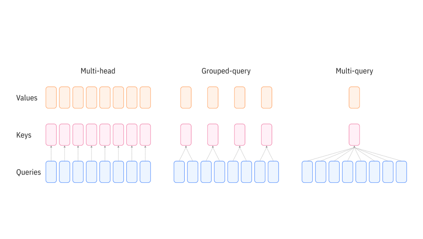
Grouped Query Attention (GQA)

GQA is an attention mechanism used in LLMs that acts as a "middle ground" between two other methods: Multi-Head Attention (MHA) and Multi-Query Attention (MQA). (Bergmann & Stryker, n.d.) Its primary goal is to achieve the high quality of MHA while getting close to the high speed and low memory usage of MQA, especially during inference (when the model is generating text). MHA dates to everyone's favorite paper "Attention is all you need". This is the standard, high-quality method. In MHA, each query head gets its own set of "key" (K) and "value" (V) heads. This is very effective but slow and memory-hungry, as it has to store same number of sets of keys and values as queries. GPUs don't have much on-board memory to store the outputs of the massive quantity of intermediate calculations that must be recalled at each subsequent processing step. Multi-query attention is a more computationally efficient attention mechanism that simplifies multi-head attention to reduce memory usage and intermediate calculations. Instead of training a unique key head and value head for each attention head, MQA uses a single key head and single value head at each layer. Therefore, key vectors and value vectors are calculated only once; this single set of key and value vectors is then shared across all attention heads. This drastically speeds up inference and saves memory, but can sometimes reduce the model's accuracy. Grouped Query Attention is the balanced compromise. It can be thought of as a flexible formulation of multi-query attention that partitions query heads into multiple groups that each share a set of keys and values, rather than sharing one set of keys and values across all query heads. GQA is also a good choice if you need to run a model on multiple GPUs. It allows to take advantage of tensor parallelism which means, that each GPU takes one group and can immediately calculate result without replicating any K/V heads across all computational units.

SwiGLU activation function

SwiGLU is a high-performance activation function that has become a standard choice in the feed-forward networks of modern large language models. It stands for Swish-Gated Linear Unit. As the name suggest it is composed of two parts - a swish function and Gated Linear Unit (GLU). (Selssabil, n.d.)

\text{swish}(x)=x\:\text{sigmoid}(\beta x) = \dfrac{x}{1 + e^{-\beta x}}

$\beta$ is a trainable parameter, but for the most part it is omitted by setting it to 1 which simplifies the equation to $\text{swish}(x)=x\:\text{sigmoid}(x)$ which is equivalent to the Sigmoid Linear Unit or SiLU. Idea behind GLU function is that it takes the output of a linear transformation and splits it into two parts: one part is passed through another linear transformation, while the second is passed through a sigmoid activation function. This enables the network to focus on important features by either blocking or passing information (similar concept as in LSTMs).

GLU(x,W,V,b,c)=\text{sigmoid}(xW+b)\times(xV+c)

SwiGLU activation function can be expressed as:

SwiGLU(x,W,V,b,c)=\text{swish}_{\beta}(xW+b)\times(xV + c)

Entire feed-forward block can be easily implemented like this:

class MLP(nn.Module):
    def __init__(self, config: Qwen3Config):
        super().__init__()
        self.gate_proj = nn.Linear(config.hidden_size, config.intermediate_size, bias=False)
        self.up_proj = nn.Linear(config.hidden_size, config.intermediate_size, bias=False)
        self.down_proj = nn.Linear(config.intermediate_size, config.hidden_size, bias=False)
        self.activation = nn.SiLU()

    def forward(self, x):
        return self.down_proj(self.activation(self.gate_proj(x)) * self.up_proj(x))

Important detail from Qwen3 paper is, that we do not use biases in any layers, therefore you can set bias=False.

Rotary Positional Embeddings (RoPE)

Rotary Positional Embeddings (RoPE) are a modern and efficient method for letting a language model understand the order of tokens in a sequence. Instead of adding a position number to a token's embedding (like it was proposed in the original "Attention is all you need" paper), RoPE rotates the query and key vectors.

In the real world, we won't be rotating whole vectors but we will apply many 2D rotations to pairs of dimensions for couple of reasons. Firstly, 2D rotations are parameter free, which is not the case for 3D or higher dimensions. Second of all, 2D rotations are much more efficient to calculate.

2D rotations are defined as a matrix:

\begin{pmatrix} \cos\alpha & -\sin\alpha \\ \sin\alpha & \cos\alpha \end{pmatrix}

where $\alpha$ is an angle that a vector will be rotated counter clockwise.

One of the benefits of RoPE is that we can pre-calculate lookup table values based on the maximal sequence length. In the context of smaller model it is not problematic since 32,786 is not that big of a value, but with growing context windows it is good to keep in mind memory usage of this solution.

The amount that each pair of values is rotated is given by this formula:

\omega_k=\dfrac{1}{\theta^{\frac{2k}{d}}}

$k$ is the index of a pair and $\theta$ is a parameter that we choose. For Qwen3 model it is set to one million. We need to get position of very token to be multiplied by calculated matrix (that's why we have torch.arange in the code block).

def build_rope_cache(max_seq_len, dim, base=1_000_000):
    inv_freq = 1.0 / (base ** (torch.arange(0, dim, 2, dtype=torch.int64).float() / dim))

    t = torch.arange(max_seq_len, device=inv_freq.device).float()
    freqs = torch.einsum("i,j->ij", t, inv_freq)
    return torch.cos(freqs), torch.sin(freqs)

When applying RoPE while using KV-cache mechanism (which will be covered in future blog post) it might get a bit tricky. My solution below is a bit over engineered because of this fact. I was constantly having troubles in which K and Q vectors were not rotated by the proper value. This solution mitigated that problem, but it is not as elegant as it might have been. In the future I should return to this part and try to polish it a bit more.

def apply_rope(q, k, cos_cache, sin_cache):
    kv_len = k.shape[1]
    q_len = q.shape[1]

    cos_k = cos_cache[:kv_len]
    sin_k = sin_cache[:kv_len]

    # With KV cache kv_len - q_len = kv_len - 1 which is correct index for q
    # Without KV cache (or prefill) it is equal to 0 which is also correct
    cos_q = cos_cache[kv_len - q_len : kv_len]
    sin_q = sin_cache[kv_len - q_len : kv_len]

    def rotate_half(x):
        x1 = x[..., : x.shape[-1] // 2]
        x2 = x[..., x.shape[-1] // 2 :]
        return torch.cat((-x2, x1), dim=-1)

    # Expand cos/sin to full head_dim
    cos_q_full = torch.cat((cos_q, cos_q), dim=-1).unsqueeze(0).unsqueeze(2)  # [1, q_len, 1, head_dim]
    sin_q_full = torch.cat((sin_q, sin_q), dim=-1).unsqueeze(0).unsqueeze(2)
    cos_k_full = torch.cat((cos_k, cos_k), dim=-1).unsqueeze(0).unsqueeze(2)  # [1, kv_len, 1, head_dim]
    sin_k_full = torch.cat((sin_k, sin_k), dim=-1).unsqueeze(0).unsqueeze(2)

    q_rot = q * cos_q_full + rotate_half(q) * sin_q_full
    k_rot = k * cos_k_full + rotate_half(k) * sin_k_full

    return q_rot, k_rot

RSMNorm

RMSNorm (Root Mean Square Normalization) is a simplification of the standard Layer Normalization (LayerNorm) technique used in LLMs. Its main goal is to get the same training stability as LayerNorm but be significantly faster and more computationally efficient. How does it differ from LayerNorm? LayerNorm does two things:

Re-centers: It subtracts the mean from the activations (making the mean zero).
Re-scales: It divides the activations by the standard deviation (making the variance one).

RMSNorm does only one of those things:

Re-scales: It just divides the activations by their Root Mean Square (RMS).

It completely skips the mean subtraction (re-centering) step. Re-centering is not as important to stability as re-scaling, while it is computationally more expensive.

RMSNorm is defined like this:

y_i=\dfrac{x_i}{\text{RMS}(x)}*\gamma_i \:\: \text{where} \: \: \text{RMS}(x)=\sqrt{\epsilon+\dfrac{1}{n}\sum_{i=1}^n x_{i}^{2}}

where $\gamma$ is a learnable scaling parameter.

Implementation is rather simple.

class RMSNorm(nn.Module):
    def __init__(self, hidden_size, rms_norm) -> None:
        super().__init__()
        self.weights = nn.Parameter(torch.ones(hidden_size))
        self.eps = rms_norm

    def forward(self, x: torch.Tensor):
        variance = x.pow(2).mean(-1, keepdim=True)
        norm = torch.rsqrt(variance + self.eps)
        normalized_x = x * norm * self.weights
        return normalized_x

Tie embeddings

Tied embeddings is a technique in language models where the input embedding layer and the output projection layer are forced to share the same weight matrix. In a standard language model, you have two massive weight matrices related to your vocabulary:

Input Embedding Layer: This is a lookup table (a matrix) at the beginning of the model. It converts an input token into a high-dimensional vector (different for every Qwen3 size) that represents its meaning. (with shape of vocab_size x hidden_size)
Output Projection Layer (or better knows as "LM Head" which stands for Language Modeling head): This is a linear layer at the very end of the model. It takes the final processed vector and projects it back to the size of the vocabulary, creating a logit score for every single possible token. (with shape of hidden_size x vocab_size)

First thing to notice is that vocab_size and hidden_size are rather large numbers. In Qwen3 model vocab_size = 151936 and ever for smallest model hidden_size = 1024. It means that we are already using about 0.16B times two parameters only for entering and exiting network. Second thing to notice is that both matrices are just transposes of each other. The "tied embeddings" technique is based on a simple idea: Why learn two separate, massive matrices for these two related jobs? Instead we use one matrix for both tasks. Embedding layer uses 'normal' version while LM head use transposed matrix. One question to ask is: Why are we not use an inverse of embedding matrix for output? Intuitively it makes more sense. Fists of all, inverse is a lot more complicated to compute especially for large matrices. Second of all, this matrix would have to be invertible on every iteration of training which is not guaranteed. Third of all, this approach just work if trained from scratch. Additionally, only models with parameter count of 0.6B, 1.7B and 4B use this technique. I have to guess that for larger model saving space is no longer that meaningful.

Interestingly enough, when we inspect safetensor file in which model weights are stored we can see that embedding layer and LM head are separate but their values are the same. It was probably done for compatibility with larger model which do not use tie embeddings.

Conclusions

In this post we covered some of the modern techniques used in cutting edge LLMs. They make possible to get best results from data and are effective while training and during inference. In the next post in this series i will cover some of the inference optimizations like KV-caching and speculative decoding which make LLMs output tokens at much faster pase.

References

Bergmann, D., & Stryker, C. (n.d.). What is grouped query attention (GQA)? https://www.ibm.com/think/topics/grouped-query-attention

Selssabil. (n.d.). Exploring SwiGLU : The Activation Function Powering Modern LLMs. https://medium.com/@s_boudefel/exploring-swiglu-the-activation-function-powering-modern-llms-9697f88221e7

Yang, A., Li, A., Yang, B., Zhang, B., Hui, B., Zheng, B., Yu, B., Gao, C., Huang, C., Lv, C., Zheng, C., Liu, D., Zhou, F., Huang, F., Hu, F., Ge, H., Wei, H., Lin, H., Tang, J., … Qiu, Z. (2025). Qwen3 Technical Report. https://arxiv.org/abs/2505.09388